Quant Trading for Programmers 09: From K-Lines To The First Explainable Factor Signal

Article 8 cleaned raw K-lines into unified CleanMarketBar objects. Now we can write factors.

We will not start with complexity. The first group of factors does only a few things: daily return, short moving average, long moving average, momentum, and volatility. They are simple enough to read, but still expose several key quant-engineering issues: windows, missing values, signal explanation, and test boundaries.

Factors Are Not Mysterious Formulas

A factor can first be understood as “a feature transformed from raw data into something a strategy can consume”.

For example:

• If close prices keep rising, momentum may be positive.
• If the short moving average is above the long moving average, trend may be stronger.
• If volatility is too high, even a rising price may need caution.

These are not guaranteed profit rules. They simply turn market data into engineering objects that are easier to compare.

Some terms will appear repeatedly later:

Term	Meaning in this article
K-line	Daily market record containing open, high, low, close, volume, and similar fields
Factor	A feature derived from market, financial, or other data, such as momentum, volatility, or valuation
Signal	An action hint interpreted from factors, such as observe, buy watch, or risk watch
Window	How many trading days are used when calculating a metric, such as 5-day moving average or 20-day momentum
Annualized	Convert a daily metric using about 252 trading days per year so different periods are easier to compare

Common factors can be grouped roughly like this: momentum factors ask whether prices have risen over a recent period; reversal factors ask whether short-term movement is overextended; volatility factors ask whether price swings are too large; volume and turnover factors ask whether market participation is active; valuation and quality factors depend more on financial data. Article 9 starts with momentum, moving averages, and volatility because they only depend on daily bars and connect directly to article 8.

Define Factor Points First

Chapter 9 adds app/factors.py. The core object is FactorPoint:

@dataclass(frozen=True)
class FactorPoint:
    symbol: str
    trade_date: date
    close: float
    return_1d: float | None
    ma_short: float | None
    ma_long: float | None
    momentum: float | None
    volatility: float | None
    signal: str

The None values are intentional. When there is not enough window data, moving averages, momentum, and volatility should not be forced. Many backtest bugs come from filling early missing values with 0.

Moving Averages Must Handle Windows Explicitly

Short and long moving averages use the same function:

def simple_moving_average(values: list[float], window: int) -> list[float | None]:
    if window <= 0:
        raise ValueError("window must be positive")
    out: list[float | None] = []
    running = 0.0
    for index, value in enumerate(values):
        running += value
        if index >= window:
            running -= values[index - window]
        out.append(round(running / window, 6) if index + 1 >= window else None)
    return out

This code does not use pandas, so readers can see the window calculation directly. Production code can later switch to a more efficient vectorized implementation, but the semantics should stay the same.

Returns And Volatility

Daily return starts from the second day:

def daily_returns(values: list[float]) -> list[float | None]:
    out: list[float | None] = [None]
    for previous, current in zip(values, values[1:], strict=False):
        out.append(round(current / previous - 1, 6) if previous else None)
    return out

Volatility uses a rolling window, then multiplies by 252 for annualization:

variance = sum((value - mean) ** 2 for value in sample) / (len(sample) - 1)
out.append(round(math.sqrt(variance * 252), 6))

This is not meant to predict the future. It simply gives later strategy logic a risk-aware input.

From Factors To Signals

build_factor_points() labels each day as one of three signal types:

if ma_short[index] > ma_long[index] and momentum > 0 and vol[index] < 0.45:
    signal = "buy_watch"
elif momentum < -0.08 or vol[index] >= 0.65:
    signal = "risk_watch"
else:
    signal = "observe"

This is not a trading holy grail. It is the first explicit, explainable, testable signal.

What matters more is the engineering property: why did the signal appear, can it be reproduced, and can boundary conditions be tested? If those three questions cannot be answered, extra strategy complexity becomes dangerous.

Integrated Run With Neighboring Chapters

The mainline repository now includes a runnable example that connects articles 9 to 12 using the same sample daily bars:

git clone https://github.com/ax2/zi-quant-platform.git
cd zi-quant-platform
uv sync --extra dev
uv run python -m scripts.chapter_examples factor-backtest --source sample

This command first prints the factor result for article 9, then continues into the article 10 minimal backtest, article 11 portfolio backtest, and article 12 metrics. Here is the real output for article 9:

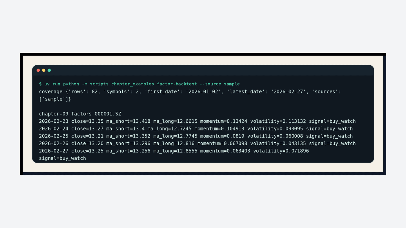
The screenshot shows that the last 5 trading days for 000001.SZ all produce buy_watch. The reason can be read directly from the fields: the short moving average is above the long moving average, 20-day momentum is positive, and annualized volatility is below the current threshold. That is the minimum standard for an explainable signal: it does not only output an action, but also explains why it appeared.

Testing Signals Matters More Than Testing Return

Chapter 9 has two important test cases.

A stable uptrend should produce buy_watch:

closes = [10 + index * 0.1 for index in range(40)]
points = build_factor_points(_bars(closes), short_window=5, long_window=20, volatility_window=5)
assert points[-1].signal == "buy_watch"

A persistent downtrend should produce risk_watch:

closes = [20 - index * 0.2 for index in range(40)]
points = build_factor_points(_bars(closes), short_window=5, long_window=20, volatility_window=5)
assert points[-1].signal == "risk_watch"

These tests do not prove the strategy can make money. They prove that trend direction, window boundaries, and risk thresholds have not been implemented backward.

Hands-On Task

Clone the chapter 9 code:

git clone https://github.com/ax2/zi-quant-platform.git
cd zi-quant-platform
git checkout chapter-09
uv sync --extra dev
uv run pytest

Run only the factor tests:

uv run pytest tests/test_factors.py

The full chapter 9 test suite passes with 164 passed, still with only the existing FastAPI deprecation warning.

Chapter Update And Repository

This chapter adds:

• app/factors.py.
• Daily return, short moving average, long moving average, momentum, annualized volatility, and three signal types.
• tests/test_factors.py, covering window boundaries, rising signals, and risk signals.
• A current-mainline scripts.chapter_examples factor-backtest integrated example that really runs the article 9-12 code path.
• Explanations for common terms such as factor, signal, window, and annualization.

Repository:

https://github.com/ax2/zi-quant-platform

Code for this chapter:

git clone https://github.com/ax2/zi-quant-platform.git
cd zi-quant-platform
git checkout chapter-09
uv sync --extra dev
uv run pytest tests/test_factors.py

Summary

Factors are not about piling up mathematical formulas. They convert market data into explainable, testable, reproducible intermediate objects.

Article 9 completes the first factor signal. The next article connects signals into the smallest backtest loop and turns them into buys, sells, cash, positions, and an equity curve.

WeChat

Follow ZiCode on WeChat

If this post was useful, you can follow later updates on WeChat as well.

X / Twitter

Follow @ax2_zicode

Faster technical notes, short thoughts, and new-post alerts are posted on X.

X Open X Profile @ax2_zicode